
Scientific computing with Python - Introduction to Pandas
Materials by Mike Hansen and Aleksandra Pawlik
There are various very useful libraries written in Python that are widely used for scientific computing. If you are unfamiliar with the concept of a "library" in programming, you can think of it as a collection of modules with functions that do specific things (for example, statistical tests) that you can call from the code you write yourself.
For example, when dealing with numeric matrices and vectors in Python, NumPy makes life a lot easier. For more complex data, however, it leaves a lot to be desired. If you're used to working with data frames in R, doing data analysis directly with NumPy feels like a step back.
Fortunately, some nice folks have written the Python Data Analysis Library (a.k.a. pandas).
Pandas provides an R-like DataFrame, produces high quality plots with matplotlib, and integrates nicely with other libraries that expect NumPy arrays.
In this tutorial, we'll go through the basics of pandas using a year's worth of weather data from Weather Underground. Pandas has a lot of functionality, so we'll only be able to cover a small fraction of what you can do. Check out the (very readable) pandas docs if you want to learn more.
The IPython Notebook file and the sample data files for this tutorial can be found in the course materials:
2014-05-08-soton/lessons/nocs/pandas/
Getting Started
OK, let's get started by importing the pandas library
import pandas
Importing a library is like getting a piece of lab equipment out of a storage locker and setting it up on the bench. Once it's done, we can ask the library to read our data file for us.
Let's read in our data then.
Because it's in a CSV file, we can use pandas' read_csv function to pull it directly into a DataFrame.
data = pandas.read_csv("data/weather_year.csv")
We can get a summary of the DataFrame by printing the object.
data
Output:
<class 'pandas.core.frame.DataFrame'>
Int64Index: 366 entries, 0 to 365
Data columns:
EDT                           366  non-null values
Max TemperatureF              366  non-null values
Mean TemperatureF             366  non-null values
Min TemperatureF              366  non-null values
Max Dew PointF                366  non-null values
MeanDew PointF                366  non-null values
Min DewpointF                 366  non-null values
Max Humidity                  366  non-null values
 Mean Humidity                366  non-null values
 Min Humidity                 366  non-null values
 Max Sea Level PressureIn     366  non-null values
 Mean Sea Level PressureIn    366  non-null values
 Min Sea Level PressureIn     366  non-null values
 Max VisibilityMiles          366  non-null values
 Mean VisibilityMiles         366  non-null values
 Min VisibilityMiles          366  non-null values
 Max Wind SpeedMPH            366  non-null values
 Mean Wind SpeedMPH           366  non-null values
 Max Gust SpeedMPH            365  non-null values
PrecipitationIn               366  non-null values
 CloudCover                   366  non-null values
 Events                       162  non-null values
 WindDirDegrees               366  non-null values
dtypes: float64(4), int64(16), object(3)
This gives us a lot of information. First, we can see that there are 366 rows (entries) – a year and a day's worth of weather. Each column is printed along with however many "non-null" values are present.
We'll talk more about null (or missing) values in pandas later, but for now we can note that only the "Max Gust SpeedMPH" and "Events" columns have fewer than 366 non-null values.
Lastly, the data types (dtypes) of the columns are printed at the very bottom. We can see that there are 4 float64, 16 int64, and 3 object columns.
len(data)
Output:
366
Using len on a DataFrame will give you the number of rows. You can get the column names using the columns property.
data.columns
Output:
Index([EDT, Max TemperatureF, Mean TemperatureF, Min TemperatureF,
       Max Dew PointF, MeanDew PointF, Min DewpointF, Max Humidity,
        Mean Humidity,  Min Humidity,  Max Sea Level PressureIn,
        Mean Sea Level PressureIn,  Min Sea Level PressureIn,
        Max VisibilityMiles,  Mean VisibilityMiles,  Min VisibilityMiles,
        Max Wind SpeedMPH,  Mean Wind SpeedMPH,  Max Gust SpeedMPH,
       PrecipitationIn,  CloudCover,  Events,  WindDirDegrees], dtype=object)
Columns can be accessed in two ways. The first is using the DataFrame like a dictionary with string keys:
data["EDT"]
Output:
0     2012-3-10
1     2012-3-11
2     2012-3-12
3     2012-3-13
4     2012-3-14
5     2012-3-15
6     2012-3-16
7     2012-3-17
8     2012-3-18
9     2012-3-19
10    2012-3-20
11    2012-3-21
12    2012-3-22
13    2012-3-23
14    2012-3-24
...
351    2013-2-24
352    2013-2-25
353    2013-2-26
354    2013-2-27
355    2013-2-28
356     2013-3-1
357     2013-3-2
358     2013-3-3
359     2013-3-4
360     2013-3-5
361     2013-3-6
362     2013-3-7
363     2013-3-8
364     2013-3-9
365    2013-3-10
Name: EDT, Length: 366
You can get multiple columns out at the same time by passing in a list of strings.
data[["EDT", "Mean TemperatureF"]]
Output:
<class 'pandas.core.frame.DataFrame'>
Int64Index: 366 entries, 0 to 365
Data columns:
EDT                  366  non-null values
Mean TemperatureF    366  non-null values
dtypes: int64(1), object(1)
The second way to access columns is using the dot syntax. This only works if your column name could also be a Python variable name (i.e., no spaces), and if it doesn't collide with another DataFrame property or function name (e.g., count, sum).
data.EDT
Output:
0     2012-3-10
1     2012-3-11
2     2012-3-12
3     2012-3-13
4     2012-3-14
5     2012-3-15
6     2012-3-16
7     2012-3-17
8     2012-3-18
9     2012-3-19
10    2012-3-20
11    2012-3-21
12    2012-3-22
13    2012-3-23
14    2012-3-24
...
351    2013-2-24
352    2013-2-25
353    2013-2-26
354    2013-2-27
355    2013-2-28
356     2013-3-1
357     2013-3-2
358     2013-3-3
359     2013-3-4
360     2013-3-5
361     2013-3-6
362     2013-3-7
363     2013-3-8
364     2013-3-9
365    2013-3-10
Name: EDT, Length: 366
We'll be mostly using the dot syntax here because you can auto-complete the names in IPython and IPython Notebook. The first pandas function we'll learn about is head(). This gives us the first 5 items in a column (or the first 5 rows in the DataFrame).
data.EDT.head()
Output:
0    2012-3-10
1    2012-3-11
2    2012-3-12
3    2012-3-13
4    2012-3-14
Name: EDT
Passing in a number n gives us the first n items in the column. There is also a corresponding tail() method that gives the last n items or rows.
data.EDT.head(10)
Output:
0    2012-3-10
1    2012-3-11
2    2012-3-12
3    2012-3-13
4    2012-3-14
5    2012-3-15
6    2012-3-16
7    2012-3-17
8    2012-3-18
9    2012-3-19
Name: EDT
This also works with the dictionary syntax.
data["Mean TemperatureF"].head()
Output:
0    40
1    49
2    62
3    63
4    62
Name: Mean TemperatureF
Exercise 1:
How would we get the second to last date (EDT) in the dataset?
# Combine head() and tail()
last_two_dates = data.EDT.tail(2)
second_to_last_date = last_two_dates.head(1)
print second_to_last_date
Output:
364    2013-3-9
Name: EDT
If the data in the column is numeric, you can use describe() to get some stats on it.
data["Mean TemperatureF"].describe()
Output:
count    366.000000
mean      55.683060
std       18.436506
min       11.000000
25%       41.000000
50%       59.000000
75%       70.750000
max       89.000000
Fun with Columns
The column names in data are a little unweildy, so we're going to rename them. You can rename individual columns with the rename() method of the DataFrame.
data = data.rename(columns={ "Max TemperatureF": "max_temp", "Min TemperatureF": "min_temp" })
data.columns
Output:
Index([EDT, max_temp, Mean TemperatureF, min_temp, Max Dew PointF,
       MeanDew PointF, Min DewpointF, Max Humidity,  Mean Humidity,
        Min Humidity,  Max Sea Level PressureIn,
        Mean Sea Level PressureIn,  Min Sea Level PressureIn,
        Max VisibilityMiles,  Mean VisibilityMiles,  Min VisibilityMiles,
        Max Wind SpeedMPH,  Mean Wind SpeedMPH,  Max Gust SpeedMPH,
       PrecipitationIn,  CloudCover,  Events,  WindDirDegrees], dtype=object)
You can see that the max and mean temperature columns are now called max_temp and mean_temp respectively.
Notice that we assigned the results of data.rename(...) to data. Most DataFrame methods do not modify the DataFrame directly, and instead return a copy or a filtered view.
Let's change all of our column names at the same time. This is as easy as assigning a new list of column names to the columns property of the DataFrame.
data.columns = ["date", "max_temp", "mean_temp", "min_temp", "max_dew",
                "mean_dew", "min_dew", "max_humidity", "mean_humidity",
                "min_humidity", "max_pressure", "mean_pressure",
                "min_pressure", "max_visibilty", "mean_visibility",
                "min_visibility", "max_wind", "mean_wind", "min_wind",
                "precipitation", "cloud_cover", "events", "wind_dir"]
These should be in the same order as the original columns. Let's take another look at our DataFrame summary.
data
Output:
<class 'pandas.core.frame.DataFrame'>
Int64Index: 366 entries, 0 to 365
Data columns:
date               366  non-null values
max_temp           366  non-null values
mean_temp          366  non-null values
min_temp           366  non-null values
max_dew            366  non-null values
mean_dew           366  non-null values
min_dew            366  non-null values
max_humidity       366  non-null values
mean_humidity      366  non-null values
min_humidity       366  non-null values
max_pressure       366  non-null values
mean_pressure      366  non-null values
min_pressure       366  non-null values
max_visibilty      366  non-null values
mean_visibility    366  non-null values
min_visibility     366  non-null values
max_wind           366  non-null values
mean_wind          366  non-null values
min_wind           365  non-null values
precipitation      366  non-null values
cloud_cover        366  non-null values
events             162  non-null values
wind_dir           366  non-null values
dtypes: float64(4), int64(16), object(3)
Now our columns can all be accessed using the dot syntax!
data.mean_temp.head()
Output:
0    40
1    49
2    62
3    63
4    62
Name: mean_temp
There are lots useful methods on columns, such as std() to get the standard deviation. Most of pandas' methods will happily ignore missing values like NaN.
data.mean_temp.std()
Output:
18.436505996251075
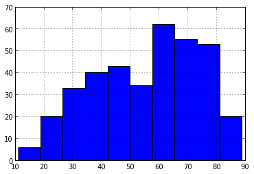
Some methods, like plot() and hist() produce plots using matplotlib. We'll go over plotting in more detail later.
data.mean_temp.hist()
Output:
<matplotlib.axes.AxesSubplot at 0x3f8a950>
By the way, many of the column-specific methods also work on the entire DataFrame. Instead of a single number, you'll get a result for each column.
data.std()
Output:
max_temp           20.361247
mean_temp          18.436506
min_temp           17.301141
max_dew            16.397178
mean_dew           16.829996
min_dew            17.479449
max_humidity        9.108438
mean_humidity       9.945591
min_humidity       15.360261
max_pressure        0.172189
mean_pressure       0.174112
min_pressure        0.182476
max_visibilty       0.073821
mean_visibility     1.875406
min_visibility      3.792219
max_wind            5.564329
mean_wind           3.200940
min_wind            8.131092
cloud_cover         2.707261
wind_dir           94.045080
If you only want to compute something over couple of the columns, use the dictionary syntax:
data[["max_temp", "max_pressure", "max_wind"]].std()
Output:
max_temp        20.361247
max_pressure     0.172189
max_wind         5.564329
Exercise 2:
What is the range of temperatures in the dataset?
Hint: columns have max() and min() methods.
hottest_temp = data.max_temp.max()  # Highest of the highs
coldest_temp = data.min_temp.min()  # Lowest of the lows
print "Temperature range:", hottest_temp - coldest_temp, "degrees F"
Output:
Temperature range: 105 degrees F
Bulk Operations with apply()
Built-on methods like sum() and std() work on entire columns. We can run our own functions across all values in a column (or row) using apply().
To give you an idea of how this works, let's consider the "date" column in our DataFrame (formally "EDT").
data.date.head()
Output:
0    2012-3-10
1    2012-3-11
2    2012-3-12
3    2012-3-13
4    2012-3-14
Name: date
We can use the values property of the column to get a list of values for the column. Inspecting the first value reveals that these are strings with a particular format.
first_date = data.date.values[0]
print first_date, "is a", type(first_date)
Output:
2012-3-10 is a <type 'str'>
The strptime function from the datetime module will make quick work of this date string. There are many more shortcuts available for strptime.
# Import the datetime class from the datetime module
from datetime import datetime

# Convert date string to datetime object
datetime.strptime(first_date, "%Y-%m-%d")
Output:
datetime.datetime(2012, 3, 10, 0, 0)
Using the apply() method, which takes a function (without the parentheses), we can apply strptime to each value in the column. We'll overwrite the string date values with their Python datetime equivalents.
	# Define a function to convert strings to dates
def string_to_date(date_string):
   	 return datetime.strptime(date_string, "%Y-%m-%d")

	# Run the function on every date string and overwrite the column
data.date = data.date.apply(string_to_date)
sdata.date.head()
Output:
0    2012-03-10 00:00:00
1    2012-03-11 00:00:00
2    2012-03-12 00:00:00
3    2012-03-13 00:00:00
4    2012-03-14 00:00:00
Name: date
Let's go one step futher. Each row in our DateFrame represents the weather from a single day. Each row in a DataFrame is associated with an index, which is a label that uniquely identifies a row.
Our row indices up to now have been auto-generated by pandas, and are simply integers from 0 to 365. If we use dates instead of integers for our index, we will get some extra benefits from pandas when plotting later on. Overwriting the index is as easy as assigning to the index property of the DataFrame.
data.index = data.date
data.index
Output:
<class 'pandas.tseries.index.DatetimeIndex'>
[2012-03-10 00:00:00, ..., 2013-03-10 00:00:00]
Length: 366, Freq: None, Timezone: None
Now we can quickly look up a row by its date with the ix[] property.
data.ix[datetime(2012, 8, 19)]
We can even slice out a while month using a list-like syntax:
data[datetime(2012, 4, 1):datetime(2012, 4, 30)]
Output:
<class 'pandas.core.frame.DataFrame'>
DatetimeIndex: 30 entries, 2012-04-01 00:00:00 to 2012-04-30 00:00:00
Data columns:
date               30  non-null values
max_temp           30  non-null values
mean_temp          30  non-null values
min_temp           30  non-null values
max_dew            30  non-null values
mean_dew           30  non-null values
min_dew            30  non-null values
max_humidity       30  non-null values
mean_humidity      30  non-null values
min_humidity       30  non-null values
max_pressure       30  non-null values
mean_pressure      30  non-null values
min_pressure       30  non-null values
max_visibilty      30  non-null values
mean_visibility    30  non-null values
min_visibility     30  non-null values
max_wind           30  non-null values
mean_wind          30  non-null values
min_wind           30  non-null values
precipitation      30  non-null values
cloud_cover        30  non-null values
events             14  non-null values
wind_dir           30  non-null values
dtypes: float64(4), int64(16), object(3)
With all of the dates in the index now, we no longer need the "date" column. Let's drop it.
data = data.drop("date", axis=1)
data.columns
Output:
Index([max_temp, mean_temp, min_temp, max_dew, mean_dew, min_dew,
       max_humidity, mean_humidity, min_humidity, max_pressure,
       mean_pressure, min_pressure, max_visibilty, mean_visibility,
       min_visibility, max_wind, mean_wind, min_wind, precipitation,
       cloud_cover, events, wind_dir], dtype=object)
Note that we need to pass in axis=1 in order to drop a column. For more details, check out the documentation for drop.
pandas.DataFrame.drop?
Exercise 3:
Print out the cloud cover for each day in May.
Hint: you can make datetime objects with the datetime(year, month, day) function
datetime(2012, 5, 1)  # May 1st of 2012


data[datetime(2012, 5, 1):datetime(2012, 5, 31)].cloud_cover
Output:
date
2012-05-01    6
2012-05-02    1
2012-05-03    0
2012-05-04    6
2012-05-05    3
2012-05-06    0
2012-05-07    5
2012-05-08    4
2012-05-09    3
2012-05-10    1
2012-05-11    0
2012-05-12    1
2012-05-13    4
2012-05-14    4
2012-05-15    0
2012-05-16    0
2012-05-17    0
2012-05-18    0
2012-05-19    0
2012-05-20    1
2012-05-21    4
2012-05-22    2
2012-05-23    0
2012-05-24    0
2012-05-25    2
2012-05-26    0
2012-05-27    0
2012-05-28    0
2012-05-29    4
2012-05-30    1
2012-05-31    4
Name: cloud_cover
Handling Missing Values
Pandas considers values like NaN and None to represent missing data. The pandas.isnull function can be used to tell whether or not a value is missing.
Let's use apply() across all of the columns in our DataFrame to figure out which values are missing.
empty = data.apply(lambda col: pandas.isnull(col))
empty
Output:
<class 'pandas.core.frame.DataFrame'>
DatetimeIndex: 366 entries, 2012-03-10 00:00:00 to 2013-03-10 00:00:00
Freq: D
Data columns:
max_temp           366  non-null values
mean_temp          366  non-null values
min_temp           366  non-null values
max_dew            366  non-null values
mean_dew           366  non-null values
min_dew            366  non-null values
max_humidity       366  non-null values
mean_humidity      366  non-null values
min_humidity       366  non-null values
max_pressure       366  non-null values
mean_pressure      366  non-null values
min_pressure       366  non-null values
max_visibilty      366  non-null values
mean_visibility    366  non-null values
min_visibility     366  non-null values
max_wind           366  non-null values
mean_wind          366  non-null values
min_wind           366  non-null values
precipitation      366  non-null values
cloud_cover        366  non-null values
events             366  non-null values
wind_dir           366  non-null values
dtypes: bool(22)
We got back a dataframe (empty) with boolean values for all 22 columns and 366 rows. Inspecting the first 10 values of the "events", column we can see that there are some missing values because a True was returned from pandas.isnull.
empty.events.head(10)
Output:
date
2012-03-10     True
2012-03-11    False
2012-03-12    False
2012-03-13     True
2012-03-14     True
2012-03-15    False
2012-03-16     True
2012-03-17    False
2012-03-18    False
2012-03-19     True
Freq: D, Name: events
Looking at the corresponding rows in the original DataFrame reveals that pandas has filled in NaN for empty values in the "events" column.
data.events.head(10)
Output:
date
2012-03-10                  NaN
2012-03-11                 Rain
2012-03-12                 Rain
2012-03-13                  NaN
2012-03-14                  NaN
2012-03-15    Rain-Thunderstorm
2012-03-16                  NaN
2012-03-17     Fog-Thunderstorm
2012-03-18                 Rain
2012-03-19                  NaN
Freq: D, Name: events
This isn't exactly what we want. One option is to drop all rows in the DataFrame with missing "events" values.
data.dropna(subset=["events"])
Output:
<class 'pandas.core.frame.DataFrame'>
DatetimeIndex: 162 entries, 2012-03-11 00:00:00 to 2013-03-06 00:00:00
Data columns:
max_temp           162  non-null values
mean_temp          162  non-null values
min_temp           162  non-null values
max_dew            162  non-null values
mean_dew           162  non-null values
min_dew            162  non-null values
max_humidity       162  non-null values
mean_humidity      162  non-null values
min_humidity       162  non-null values
max_pressure       162  non-null values
mean_pressure      162  non-null values
min_pressure       162  non-null values
max_visibilty      162  non-null values
mean_visibility    162  non-null values
min_visibility     162  non-null values
max_wind           162  non-null values
mean_wind          162  non-null values
min_wind           162  non-null values
precipitation      162  non-null values
cloud_cover        162  non-null values
events             162  non-null values
wind_dir           162  non-null values
dtypes: float64(4), int64(16), object(2)
The DataFrame we get back has only 162 rows, so we can infer that there were 366 - 162 = 204 missing values in the "events" column. Note that this didn't affect data; we're just looking at a copy.
Instead of dropping the rows with missing values, let's fill them with empty strings (you'll see why in a moment). This is easily done with the fillna() function. We'll go ahead and overwrite the "events" column with empty string missing values instead of NaN.
data.events = data.events.fillna("")
data.events.head(10)
Output:
date
2012-03-10
2012-03-11                 Rain
2012-03-12                 Rain
2012-03-13
2012-03-14
2012-03-15    Rain-Thunderstorm
2012-03-16
2012-03-17     Fog-Thunderstorm
2012-03-18                 Rain
2012-03-19
Freq: D, Name: events
Accessing Individual Rows
Sometimes you need to access individual rows in your DataFrame. The irow() function lets you grab the ith row from a DataFrame (starting from 0).
data.irow(0)
Output:
max_temp              56
mean_temp             40
min_temp              24
max_dew               24
mean_dew              20
min_dew               16
max_humidity          74
mean_humidity         50
min_humidity          26
max_pressure       30.53
mean_pressure      30.45
min_pressure       30.34
max_visibilty         10
mean_visibility       10
min_visibility        10
max_wind              13
mean_wind              6
min_wind              17
precipitation       0.00
cloud_cover            0
events
wind_dir             138
Name: 2012-03-10 00:00:00
Of course, another option is to use the index.
data.ix[datetime(2013, 1, 1)]
Output:
max_temp              32
mean_temp             26
min_temp              20
max_dew               31
mean_dew              25
min_dew               16
max_humidity          92
mean_humidity         83
min_humidity          74
max_pressure        30.2
mean_pressure      30.11
min_pressure       30.04
max_visibilty          9
mean_visibility        5
min_visibility         2
max_wind              14
mean_wind              5
min_wind              15
precipitation          T
cloud_cover            8
events
wind_dir             353
Name: 2013-01-01 00:00:00
You can iterate over each row in the DataFrame with iterrows(). Note that this function returns both the index and the row. Also, you must access columns in the row you get back from iterrows() with the dictionary syntax.
num_rain = 0
for idx, row in data.iterrows():
	if "Rain" in row["events"]:
    	num_rain += 1

print "Days with rain:", num_rain
Output:
Days with rain: 121
Exercise 4:
Was there any November rain?
Hint: check out the strftime() function on datetime objects and the documentation
d = datetime(2012, 1, 1)
d.strftime("%B")


november_rain = False
for date_idx, row in data.iterrows():
	if date_idx.strftime("%B") == "November" and "Rain" in row["events"]:
    november_rain = True

if november_rain:
	print "There was rain in November"
else:
	print "There was *not* rain in November"
Output:
There was rain in November
Filtering
Most of your time using pandas will likely be devoted to selecting rows of interest from a DataFrame. In addition to strings, the dictionary syntax accepts things like this:
freezing_days = data[data.max_temp <= 32]
freezing_days
Output:
<class 'pandas.core.frame.DataFrame'>
DatetimeIndex: 21 entries, 2012-11-24 00:00:00 to 2013-03-06 00:00:00
Data columns:
max_temp           21  non-null values
mean_temp          21  non-null values
min_temp           21  non-null values
max_dew            21  non-null values
mean_dew           21  non-null values
min_dew            21  non-null values
max_humidity       21  non-null values
mean_humidity      21  non-null values
min_humidity       21  non-null values
max_pressure       21  non-null values
mean_pressure      21  non-null values
min_pressure       21  non-null values
max_visibilty      21  non-null values
mean_visibility    21  non-null values
min_visibility     21  non-null values
max_wind           21  non-null values
mean_wind          21  non-null values
min_wind           21  non-null values
precipitation      21  non-null values
cloud_cover        21  non-null values
events             21  non-null values
wind_dir           21  non-null values
dtypes: float64(4), int64(16), object(2)
We get back another DataFrame with fewer rows (21 in this case). This DataFrame can be filtered down even more.
freezing_days[freezing_days.min_temp >= 20]
Output:
<class 'pandas.core.frame.DataFrame'>
DatetimeIndex: 7 entries, 2012-11-24 00:00:00 to 2013-03-06 00:00:00
Data columns:
max_temp           7  non-null values
mean_temp          7  non-null values
min_temp           7  non-null values
max_dew            7  non-null values
mean_dew           7  non-null values
min_dew            7  non-null values
max_humidity       7  non-null values
mean_humidity      7  non-null values
min_humidity       7  non-null values
max_pressure       7  non-null values
mean_pressure      7  non-null values
min_pressure       7  non-null values
max_visibilty      7  non-null values
mean_visibility    7  non-null values
min_visibility     7  non-null values
max_wind           7  non-null values
mean_wind          7  non-null values
min_wind           7  non-null values
precipitation      7  non-null values
cloud_cover        7  non-null values
events             7  non-null values
wind_dir           7  non-null values
dtypes: float64(4), int64(16), object(2)
Or, using boolean operations, we could apply both filters to the original DataFrame at the same time.
data[(data.max_temp <= 32) & (data.min_temp >= 20)]
Output:
<class 'pandas.core.frame.DataFrame'>
DatetimeIndex: 7 entries, 2012-11-24 00:00:00 to 2013-03-06 00:00:00
Data columns:
max_temp           7  non-null values
mean_temp          7  non-null values
min_temp           7  non-null values
max_dew            7  non-null values
mean_dew           7  non-null values
min_dew            7  non-null values
max_humidity       7  non-null values
mean_humidity      7  non-null values
min_humidity       7  non-null values
max_pressure       7  non-null values
mean_pressure      7  non-null values
min_pressure       7  non-null values
max_visibilty      7  non-null values
mean_visibility    7  non-null values
min_visibility     7  non-null values
max_wind           7  non-null values
mean_wind          7  non-null values
min_wind           7  non-null values
precipitation      7  non-null values
cloud_cover        7  non-null values
events             7  non-null values
wind_dir           7  non-null values
dtypes: float64(4), int64(16), object(2)
It's important to understand what's really going on underneath with filtering. Let's look at what kind of object we actually get back when creating a filter.
temp_max = data.max_temp <= 32
type(temp_max)
Output:
pandas.core.series.TimeSeries
This is a pandas Series object, which is the one-dimensional equivalent of a DataFrame. Because our DataFrame uses datetime objects for the index, we have a specialized TimeSeries object.
What's inside the filter?
temp_max
Output:
date
2012-03-10    False
2012-03-11    False
2012-03-12    False
2012-03-13    False
2012-03-14    False
2012-03-15    False
2012-03-16    False
2012-03-17    False
2012-03-18    False
2012-03-19    False
2012-03-20    False
2012-03-21    False
2012-03-22    False
2012-03-23    False
2012-03-24    False
...
2013-02-24    False
2013-02-25    False
2013-02-26    False
2013-02-27    False
2013-02-28    False
2013-03-01    False
2013-03-02     True
2013-03-03    False
2013-03-04    False
2013-03-05    False
2013-03-06     True
2013-03-07    False
2013-03-08    False
2013-03-09    False
2013-03-10    False
Freq: D, Name: max_temp, Length: 366
Our filter is nothing more than a Series with a boolean value for every item in the index. When we "run the filter" as so:
data[temp_max]
Output:
<class 'pandas.core.frame.DataFrame'>
DatetimeIndex: 21 entries, 2012-11-24 00:00:00 to 2013-03-06 00:00:00
Data columns:
max_temp           21  non-null values
mean_temp          21  non-null values
min_temp           21  non-null values
max_dew            21  non-null values
mean_dew           21  non-null values
min_dew            21  non-null values
max_humidity       21  non-null values
mean_humidity      21  non-null values
min_humidity       21  non-null values
max_pressure       21  non-null values
mean_pressure      21  non-null values
min_pressure       21  non-null values
max_visibilty      21  non-null values
mean_visibility    21  non-null values
min_visibility     21  non-null values
max_wind           21  non-null values
mean_wind          21  non-null values
min_wind           21  non-null values
precipitation      21  non-null values
cloud_cover        21  non-null values
events             21  non-null values
wind_dir           21  non-null values
dtypes: float64(4), int64(16), object(2)
pandas lines up the rows of the DataFrame and the filter using the index, and then keeps the rows with a True filter value. That's it.
Let's create another filter.
temp_min = data.min_temp >= 20
temp_min
Output:
date
2012-03-10    True
2012-03-11    True
2012-03-12    True
2012-03-13    True
2012-03-14    True
2012-03-15    True
2012-03-16    True
2012-03-17    True
2012-03-18    True
2012-03-19    True
2012-03-20    True
2012-03-21    True
2012-03-22    True
2012-03-23    True
2012-03-24    True
...
2013-02-24     True
2013-02-25     True
2013-02-26     True
2013-02-27     True
2013-02-28     True
2013-03-01     True
2013-03-02     True
2013-03-03    False
2013-03-04    False
2013-03-05     True
2013-03-06     True
2013-03-07     True
2013-03-08     True
2013-03-09     True
2013-03-10     True
Freq: D, Name: min_temp, Length: 366
Now we can see what the boolean operations are doing. Something like & (not and)…
temp_min & temp_max
Output:
date
2012-03-10    False
2012-03-11    False
2012-03-12    False
2012-03-13    False
2012-03-14    False
2012-03-15    False
2012-03-16    False
2012-03-17    False
2012-03-18    False
2012-03-19    False
2012-03-20    False
2012-03-21    False
2012-03-22    False
2012-03-23    False
2012-03-24    False
...
2013-02-24    False
2013-02-25    False
2013-02-26    False
2013-02-27    False
2013-02-28    False
2013-03-01    False
2013-03-02     True
2013-03-03    False
2013-03-04    False
2013-03-05    False
2013-03-06     True
2013-03-07    False
2013-03-08    False
2013-03-09    False
2013-03-10    False
Freq: D, Length: 366
…is just lining up the two filters using the index, performing a boolean AND operation, and returning the result as another Series.
We can do other boolean operations too, like OR:
temp_min | temp_max
Output:
date
2012-03-10    True
2012-03-11    True
2012-03-12    True
2012-03-13    True
2012-03-14    True
2012-03-15    True
2012-03-16    True
2012-03-17    True
2012-03-18    True
2012-03-19    True
2012-03-20    True
2012-03-21    True
2012-03-22    True
2012-03-23    True
2012-03-24    True
...
2013-02-24     True
2013-02-25     True
2013-02-26     True
2013-02-27     True
2013-02-28     True
2013-03-01     True
2013-03-02     True
2013-03-03    False
2013-03-04    False
2013-03-05     True
2013-03-06     True
2013-03-07     True
2013-03-08     True
2013-03-09     True
2013-03-10     True
Freq: D, Length: 366
Because the result is just another Series, we have all of the regular pandas functions at our disposal. The any() function returns True if any value in the Series is True.
temp_both = temp_min & temp_max
temp_both.any()
Output:
True
Sometimes filters aren't so intuitive. This (sadly) doesn't work:
try:
	data["Rain" in data.events]
except:
	pass # "KeyError: no item named False"
We can wrap it up in an apply() call fairly easily, though:
def has_rain(event_string):
	return "Rain" in event_string

data[data.events.apply(has_rain)]
Output:
<class 'pandas.core.frame.DataFrame'>
DatetimeIndex: 121 entries, 2012-03-11 00:00:00 to 2013-03-05 00:00:00
Data columns:
max_temp           121  non-null values
mean_temp          121  non-null values
min_temp           121  non-null values
max_dew            121  non-null values
mean_dew           121  non-null values
min_dew            121  non-null values
max_humidity       121  non-null values
mean_humidity      121  non-null values
min_humidity       121  non-null values
max_pressure       121  non-null values
mean_pressure      121  non-null values
min_pressure       121  non-null values
max_visibilty      121  non-null values
mean_visibility    121  non-null values
min_visibility     121  non-null values
max_wind           121  non-null values
mean_wind          121  non-null values
min_wind           121  non-null values
precipitation      121  non-null values
cloud_cover        121  non-null values
events             121  non-null values
wind_dir           121  non-null values
dtypes: float64(4), int64(16), object(2)
Exercise 5:
Before starting the exercise, let's convert the precipitation column in the dataset to floating point numbers. It's currently full of strings because of the "T" value, which stands for "trace amount of precipitation."
data.precipitation.head()
Output:
date
2012-03-10    0.00
2012-03-11       T
2012-03-12    0.03
2012-03-13    0.00
2012-03-14    0.00
Freq: D, Name: precipitation
We'll replace "T" with a very small number, and convert the rest of the strings to floats:
	# Convert precipitation to floating point number
	# "T" means "trace of precipitation"
def precipitation_to_float(precip_str):
    if precip_str == "T":
        return 1e-10  # Very small value
    return float(precip_str)

data.precipitation = data.precipitation.apply(precipitation_to_float)
data.precipitation.head()
Output:
date
2012-03-10    0.000000e+00
2012-03-11    1.000000e-10
2012-03-12    3.000000e-02
2012-03-13    0.000000e+00
2012-03-14    0.000000e+00
Freq: D, Name: precipitation
Now on to the exercise.
What was the coldest it ever got when there was no cloud cover and no precipitation?
no_cloud_cover = (data.cloud_cover == 0)
no_precipitation = (data.precipitation == 0)
coldest_temp = data[no_cloud_cover & no_precipitation].min_temp.min()
print "Coldest without cloud cover and precipitation was", coldest_temp, "degree(s) F"
Output:
Coldest without cloud cover and precipitation was 1 degree(s) F
Grouping
Besides apply(), another great DataFrame function is groupby().
It will group a DataFrame by one or more columns, and let you iterate through each group.
As an example, let's group our DataFrame by the "cloud_cover" column (a value ranging from 0 to 8).
cover_temps = {}
for cover, cover_data in data.groupby("cloud_cover"):
    cover_temps[cover] = cover_data.mean_temp.mean()  # The mean mean temp!
cover_temps
Output:
{0: 59.730769230769234,
 1: 61.415094339622641,
 2: 59.727272727272727,
 3: 58.0625,
 4: 51.5,
 5: 50.827586206896555,
 6: 57.727272727272727,
 7: 46.5,
 8: 40.909090909090907}
When you iterate through the result of groupby(), you will get a tuple.
The first item is the column value, and the second item is a filtered DataFrame (where the column equals the first tuple value).
You can group by more than one column as well.
In this case, the first tuple item returned by groupby() will itself be a tuple with the value of each column.
for (cover, events), group_data in data.groupby(["cloud_cover", "events"]):
    print "Cover: {0}, Events: {1}, Count: {2}".format(cover, events, len(group_data))
Output:
Cover: 0, Events: , Count: 99
Cover: 0, Events: Fog, Count: 2
Cover: 0, Events: Rain, Count: 2
Cover: 0, Events: Thunderstorm, Count: 1
Cover: 1, Events: , Count: 35
Cover: 1, Events: Fog, Count: 5
Cover: 1, Events: Fog-Rain, Count: 1
Cover: 1, Events: Rain, Count: 4
Cover: 1, Events: Rain-Thunderstorm, Count: 2
Cover: 1, Events: Thunderstorm, Count: 6
Cover: 2, Events: , Count: 20
Cover: 2, Events: Fog, Count: 1
Cover: 2, Events: Rain, Count: 5
Cover: 2, Events: Rain-Thunderstorm, Count: 4
Cover: 2, Events: Snow, Count: 1
Cover: 2, Events: Thunderstorm, Count: 2
Cover: 3, Events: , Count: 12
Cover: 3, Events: Fog, Count: 2
Cover: 3, Events: Fog-Rain-Thunderstorm, Count: 3
Cover: 3, Events: Fog-Thunderstorm, Count: 1
Cover: 3, Events: Rain, Count: 9
Cover: 3, Events: Rain-Thunderstorm, Count: 4
Cover: 3, Events: Snow, Count: 1
Cover: 4, Events: , Count: 16
Cover: 4, Events: Fog, Count: 3
Cover: 4, Events: Fog-Rain, Count: 2
Cover: 4, Events: Fog-Rain-Thunderstorm, Count: 2
Cover: 4, Events: Rain, Count: 10
Cover: 4, Events: Rain-Thunderstorm, Count: 6
Cover: 4, Events: Snow, Count: 1
Cover: 5, Events: , Count: 9
Cover: 5, Events: Fog-Rain, Count: 1
Cover: 5, Events: Fog-Rain-Snow, Count: 1
Cover: 5, Events: Rain, Count: 13
Cover: 5, Events: Rain-Thunderstorm, Count: 3
Cover: 5, Events: Snow, Count: 2
Cover: 6, Events: , Count: 3
Cover: 6, Events: Fog-Rain, Count: 2
Cover: 6, Events: Fog-Rain-Snow, Count: 1
Cover: 6, Events: Fog-Rain-Thunderstorm, Count: 2
Cover: 6, Events: Rain, Count: 9
Cover: 6, Events: Rain-Thunderstorm, Count: 4
Cover: 6, Events: Snow, Count: 1
Cover: 7, Events: , Count: 5
Cover: 7, Events: Fog-Rain, Count: 1
Cover: 7, Events: Fog-Rain-Thunderstorm, Count: 1
Cover: 7, Events: Fog-Snow, Count: 3
Cover: 7, Events: Rain, Count: 6
Cover: 7, Events: Rain-Thunderstorm, Count: 3
Cover: 7, Events: Snow, Count: 1
Cover: 8, Events: , Count: 5
Cover: 8, Events: Fog-Rain, Count: 4
Cover: 8, Events: Fog-Rain-Snow, Count: 1
Cover: 8, Events: Fog-Rain-Snow-Thunderstorm, Count: 1
Cover: 8, Events: Fog-Snow, Count: 2
Cover: 8, Events: Rain, Count: 11
Cover: 8, Events: Rain-Snow, Count: 3
Cover: 8, Events: Snow, Count: 6
Creating New Columns
Weather events in our DataFrame are stored in strings like "Rain-Thunderstorm" to represent that it rained and there was a thunderstorm that day. Let's split them out into boolean "rain", "thunderstorm", etc. columns.
First, let's discover the different kinds of weather events we have with unique().
data.events.unique()
Output:
array([, Rain, Rain-Thunderstorm, Fog-Thunderstorm, Fog-Rain, Thunderstorm,
       Fog-Rain-Thunderstorm, Fog, Fog-Rain-Snow,
       Fog-Rain-Snow-Thunderstorm, Fog-Snow, Snow, Rain-Snow], dtype=object)
Looks like we have "Rain", "Thunderstorm", "Fog", and "Snow" events. Creating a new column for each of these event kinds is a piece of cake with the dictionary syntax.
for event_kind in ["Rain", "Thunderstorm", "Fog", "Snow"]:
    col_name = event_kind.lower()  # Turn "Rain" into "rain", etc.
    data[col_name] = data.events.apply(lambda e: event_kind in e)
data
Output:
<class 'pandas.core.frame.DataFrame'>
DatetimeIndex: 366 entries, 2012-03-10 00:00:00 to 2013-03-10 00:00:00
Freq: D
Data columns:
max_temp           366  non-null values
mean_temp          366  non-null values
min_temp           366  non-null values
max_dew            366  non-null values
mean_dew           366  non-null values
min_dew            366  non-null values
max_humidity       366  non-null values
mean_humidity      366  non-null values
min_humidity       366  non-null values
max_pressure       366  non-null values
mean_pressure      366  non-null values
min_pressure       366  non-null values
max_visibilty      366  non-null values
mean_visibility    366  non-null values
min_visibility     366  non-null values
max_wind           366  non-null values
mean_wind          366  non-null values
min_wind           365  non-null values
precipitation      366  non-null values
cloud_cover        366  non-null values
events             366  non-null values
wind_dir           366  non-null values
rain               366  non-null values
thunderstorm       366  non-null values
fog                366  non-null values
snow               366  non-null values
dtypes: bool(4), float64(5), int64(16), object(1)
Our new columns show up at the bottom. We can access them now with the dot syntax.
data.rain
Output:
date
2012-03-10    False
2012-03-11     True
2012-03-12     True
2012-03-13    False
2012-03-14    False
2012-03-15     True
2012-03-16    False
2012-03-17    False
2012-03-18     True
2012-03-19    False
2012-03-20    False
2012-03-21    False
2012-03-22     True
2012-03-23     True
2012-03-24     True
...
2013-02-24    False
2013-02-25    False
2013-02-26     True
2013-02-27    False
2013-02-28     True
2013-03-01    False
2013-03-02    False
2013-03-03    False
2013-03-04     True
2013-03-05     True
2013-03-06    False
2013-03-07    False
2013-03-08    False
2013-03-09    False
2013-03-10    False
Freq: D, Name: rain, Length: 366
We can also do cool things like find out how many True values there are (i.e., how many days had rain)…
data.rain.sum()
Output:
121
…and get all the days that had both rain and snow!
data[data.rain & data.snow]
Output:
<class 'pandas.core.frame.DataFrame'>
DatetimeIndex: 7 entries, 2012-11-12 00:00:00 to 2013-03-05 00:00:00
Data columns:
max_temp           7  non-null values
mean_temp          7  non-null values
min_temp           7  non-null values
max_dew            7  non-null values
mean_dew           7  non-null values
min_dew            7  non-null values
max_humidity       7  non-null values
mean_humidity      7  non-null values
min_humidity       7  non-null values
max_pressure       7  non-null values
mean_pressure      7  non-null values
min_pressure       7  non-null values
max_visibilty      7  non-null values
mean_visibility    7  non-null values
min_visibility     7  non-null values
max_wind           7  non-null values
mean_wind          7  non-null values
min_wind           7  non-null values
precipitation      7  non-null values
cloud_cover        7  non-null values
events             7  non-null values
wind_dir           7  non-null values
rain               7  non-null values
thunderstorm       7  non-null values
fog                7  non-null values
snow               7  non-null values
dtypes: bool(4), float64(5), int64(16), object(1)
Exercise 6:
Was the mean temperature more variable on days with rain and snow than on days with just rain or just snow?
Hint: don't forget the std() function
days_with_rain = data[data.rain == True]
days_with_snow = data[data.snow == True]

rain_std = days_with_rain.mean_temp.std()
snow_std = days_with_snow.mean_temp.std()

if rain_std > snow_std:
    print "Rainy days were more variable"
elif snow_std > rain_std:
    print "Snowy days were more variable"
else:
    print "They were the same"
Output:
Rainy days were more variable
Plotting
We've already seen how the hist() function makes generating histograms a snap. Let's look at the plot() function now.
data.max_temp.plot()
Output:
<matplotlib.axes.AxesSubplot at 0x46f2610>
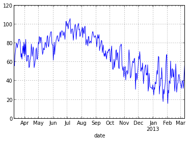
That one line of code did a lot for us. First, it created a nice looking line plot using the maximum temperature column from our DataFrame. Second, because we used datetime objects in our index, pandas labeled the x-axis appropriately.
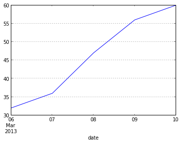
Pandas is smart too. If we're only looking at a couple of days, the x-axis looks different:
data.max_temp.tail().plot()
Output:
<matplotlib.axes.AxesSubplot at 0x4c03710>
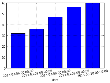
Prefer a bar plot? Pandas has got your covered.
data.max_temp.tail().plot(kind="bar", rot=10)
Output:
<matplotlib.axes.AxesSubplot at 0x4e803d0>
The plot() function returns a matplotlib AxesSubPlot object. You can pass this object into subsequent calls to plot() in order to compose plots.
Although plot() takes a variety of parameters to customize your plot, users familiar with matplotlib will feel right at home with the AxesSubPlot object.
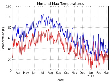
ax = data.max_temp.plot(title="Min and Max Temperatures")
data.min_temp.plot(style="red", ax=ax)
ax.set_ylabel("Temperature (F)")
Output:
<matplotlib.text.Text at 0x50f0f90>
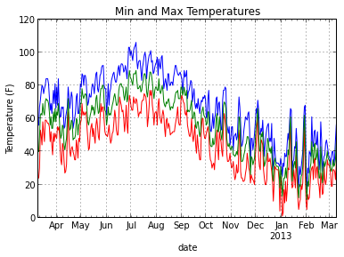
Exercise 7:
Add the mean temperature to the previous plot using a green line. Also, add a legend with the legend() method of ax.
ax = data.max_temp.plot(title="Min and Max Temperatures")
data.min_temp.plot(style="red", ax=ax)
data.mean_temp.plot(style="green", ax=ax)
ax.set_ylabel("Temperature (F)")
Output:
<matplotlib.text.Text at 0x532ec90>
Getting Data Out
Writing data out in pandas is as easy as getting data in. To save our DataFrame out to a new csv file, we can just do this:
data.to_csv("data/weather-mod.csv")
Want to make that tab separated instead? No problem.
data.to_csv("data/weather-mod.tsv", sep="\t")
There's also support for reading and writing Excel files, if you need it.
Miscellanea
We've only covered a small fraction of the pandas library here. Before I wrap up, however, there are a few miscellaneous tips I'd like to go over.
First, it can be confusing to know when an operation will modify a DataFrame and when it will return a copy to you. Pandas behavior here is entirely dictated by NumPy, and some situations are unintuitive.
For example, what do you think will happen here?
for idx, row in data.iterrows():
	row["max_temp"] = 0
data.max_temp.head()
Output:
date
2012-03-10    56
2012-03-11    67
2012-03-12    71
2012-03-13    76
2012-03-14    80
Freq: D, Name: max_temp
Contrary to what you might expect, modifying row did not modify data!
This is because row is a copy, and does not point back to the original DataFrame.
Here's the right way to do it:
for idx, row in data.iterrows():
    data.ix[idx, "max_temp"] = 0
any(data.max_temp != 0)  # Any rows with max_temp not equal to zero?
Output:
False
Just to make you even more confused, this also doesn't work:
for idx, row in data.iterrows():
    data.ix[idx]["max_temp"] = 100
data.max_temp.head()
Output:
date
2012-03-10    0
2012-03-11    0
2012-03-12    0
2012-03-13    0
2012-03-14    0
Freq: D, Name: max_temp
When using apply(), the default behavior is to go over columns.
data.apply(lambda c: c.name)
Output:
max_temp                  max_temp
mean_temp                mean_temp
min_temp                  min_temp
max_dew                    max_dew
mean_dew                  mean_dew
min_dew                    min_dew
max_humidity          max_humidity
mean_humidity        mean_humidity
min_humidity          min_humidity
max_pressure          max_pressure
mean_pressure        mean_pressure
min_pressure          min_pressure
max_visibilty        max_visibilty
mean_visibility    mean_visibility
min_visibility      min_visibility
max_wind                  max_wind
mean_wind                mean_wind
min_wind                  min_wind
precipitation        precipitation
cloud_cover            cloud_cover
events                      events
wind_dir                  wind_dir
rain                          rain
thunderstorm          thunderstorm
fog                            fog
snow                          snow
You can make apply() go over rows by passing axis=1
data.apply(lambda r: r["max_pressure"] - r["min_pressure"], axis=1)
Output:
date
2012-03-10    0.19
2012-03-11    0.24
2012-03-12    0.25
2012-03-13    0.15
2012-03-14    0.11
2012-03-15    0.11
2012-03-16    0.07
2012-03-17    0.11
2012-03-18    0.12
2012-03-19    0.11
2012-03-20    0.10
2012-03-21    0.12
2012-03-22    0.10
2012-03-23    0.27
2012-03-24    0.09
...
2013-02-24    0.15
2013-02-25    0.33
2013-02-26    0.40
2013-02-27    0.23
2013-02-28    0.28
2013-03-01    0.11
2013-03-02    0.11
2013-03-03    0.08
2013-03-04    0.20
2013-03-05    0.26
2013-03-06    0.53
2013-03-07    0.13
2013-03-08    0.13
2013-03-09    0.36
2013-03-10    0.05
Length: 366
When you call drop(), though, it's flipped. To drop a column, you need to pass axis=1
data.drop(["events"], axis=1).columns
Output:
Index([max_temp, mean_temp, min_temp, max_dew, mean_dew, min_dew,
       max_humidity, mean_humidity, min_humidity, max_pressure,
       mean_pressure, min_pressure, max_visibilty, mean_visibility,
       min_visibility, max_wind, mean_wind, min_wind, precipitation,
       cloud_cover, wind_dir, rain, thunderstorm, fog, snow], dtype=object)